Exploring Ouroboros with wireshark

I recently did some quick tests with the new congestion avoidance implementation, and thought to myself that it was a shame that Wireshark could not identify the Ouroboros flows, as that could give me some nicer graphs.

Just to be clear, I think generic network tools like tcpdump and wireshark – however informative and nice-to-use they are – are a symptom of a lack of network security. The whole point of Ouroboros is that it is intentionally designed to make it hard to analyze network traffic. Ouroboros is not a network stack¹: one can’t simply dump a packet from the wire and derive the packet contents all the way up to the application by following identifiers for protocols and well-known ports. Using encryption to hide the network structure from the packet is shutting the door after the horse has bolted.

To write an Ouroboros dissector, one needs to know the layered structure of the network at the capturing point at that specific point in time. It requires information from the Ouroboros runtime on the capturing machine and at the exact time of the capture, to correctly analyze traffic flows. I just wrote a dissector that works for my specific setup².

Congestion avoidance test

First, a quick refresh on the experiment layout, it’s the the same 4-node experiment as in the previous post

I tried to draw the setup as best as I can in the figure above.

There are 4 rack mounted 1U servers, connected over Gigabit Ethernet (GbE). Physically there is a big switch connecting all of them, but each “link” is separated as a port-based VLAN, so there are 3 independent Ethernet segments. We create 3 ethernet layers, drawn in a lighter gray, with a single unicast layer – consisting of 4 unicast IPC processes (IPCPs) – on top, drawn in a darker shade of gray. The link between the router and server has been capped to 100 megabit/s using ethtool³, and traffic is captured on the Ethernet NIC at the “Server” node using tcpdump. All traffic is generated with our constant bit rate ocbr tool trying to send about 80 Mbit/s of application-level throughput over the unicast layer.

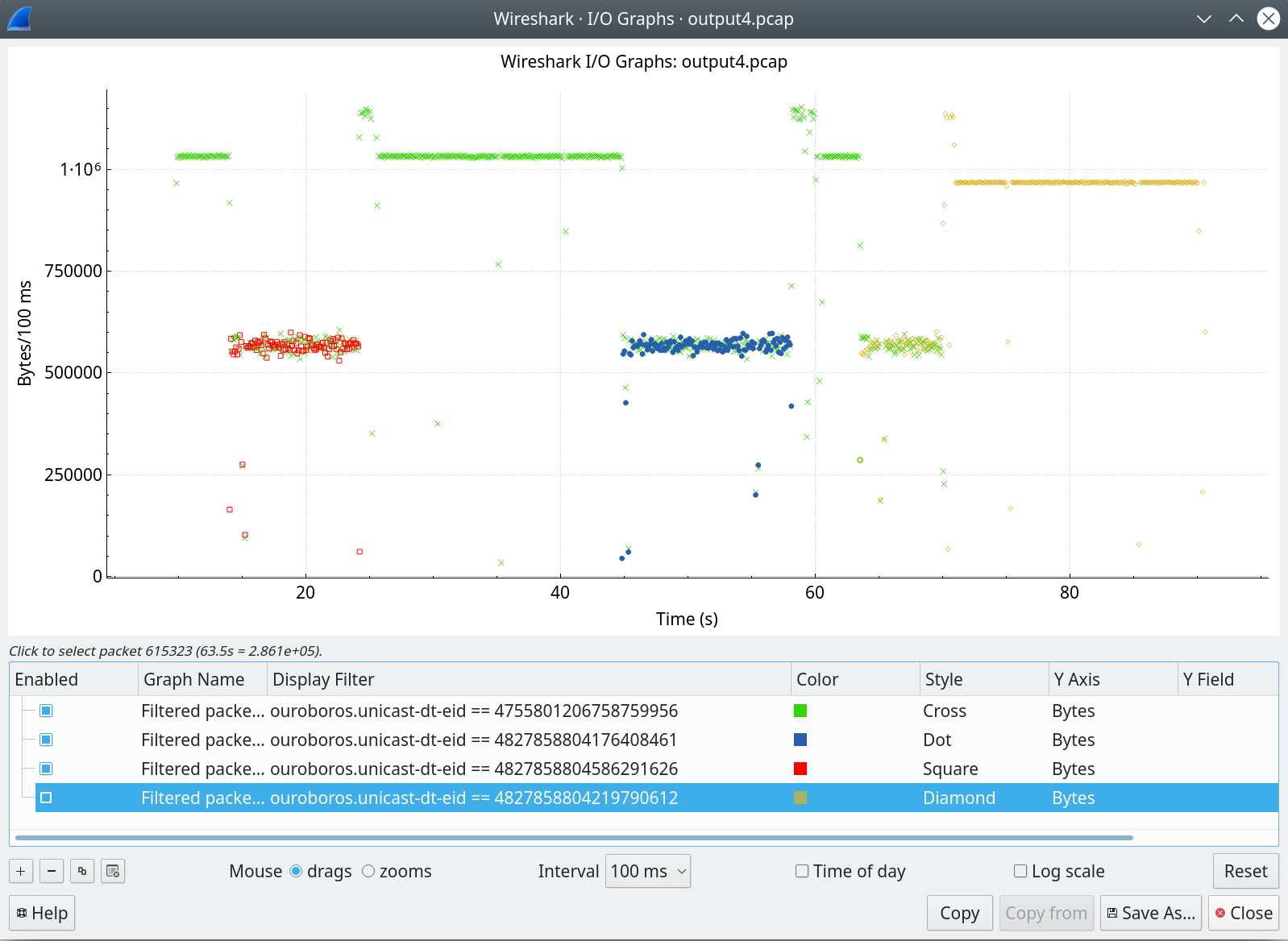
The graph above shows the bandwidth – as captured on the congested 100Mbit Ethernet link –, separated for each traffic flow, from the same pcap capture as in my previous post. A flow can be identified by a (destination address, endpoint ID)-pair, and since the destination is all the same, I could filter out the flows by simply selecting them based on the (64-bit) endpoint identifier.

What you’re looking at is that first, a flow (green starts), at around T=14s, a new flow enters (red) that stops at around T=24s. At around T=44s, another flow enters (blue) for about 14 seconds, and finally, a fourth (orange) flow enters at T=63s. The first (green) flow exits at around T=70s, leaving all the available bandwidth for the orange flow.

The most important thing that I wanted to check is that when there are multiple flows, if and how fast they would converge to the same bandwidth. I’m not dissatisfied with the initial result: the answers seem to be yes and pretty fast, with no observable oscillation to boot⁴

Protocol overview

Now, the wireshark dissector can be used to present some more details about the Ouroboros protocols in a familiar setting – make it more accessible to some – so, let’s have a quick look.

The Ouroboros network protocol has 5 fields:

| DST | TTL | QOS | ECN | EID |

which we had to map to the Ethernet II protocol for our ipcpd-eth-dix implementation. The basic Ethernet II MAC (layer-2) header is pretty simple. It has 2 6-byte addresses (dst, src) and a 2-byte Ethertype.

Since Ethernet doesn’t do QoS or congestion, the main missing field here is the EID. We could have mapped it to the Ethertype, but we noticed that a lot of routers and switches drop unknown Ethertypes (and, for the purposes of this blog post here: it would have all but prevented to write the dissector). So we made the ethertype configurable per layer (so it can be set to a value that is not blocked by the network), and added 2 16-bit fields after the Ethernet MAC header for an Ouroboros layer:

• Endpoint ID eid, which works just like in the unicast layer, to identify the N+1 application (in our case: a data transfer flow and a management flow for a unicast IPC process).

• A length field len, which is needed because Ethernet NICs pad frames that are smaller than 64 bytes in length with trailing zeros (and we receive these zeros in our code). A length field is present in Ethernet type I, but since most “Layer 3” protocols also had a length field, it was re-purposed as Ethertype in Ethernet II. The value of the len field is the length of the data payload.

The Ethernet layer that spans that 100Mbit link has Ethertype 0xA000 set (which is the Ouroboros default), the Ouroboros plugin hooks into that ethertype.

On top of the Ethernet layer, we have a unicast, layer with the 5 fields specified above. The dissector also shows the contents of the flow allocation messages, which are (currently) sent to EID = 0.

So, the protocol header as analysed in the experiment is, starting from the “wire”:

+---------+---------+-----------+-----+-----+------
| dst MAC | src MAC | Ethertype | eid | len | data   /* ETH LAYER */
+---------+---------+-----------+-----+-----+------

   <IF eid != 0 >       /* eid == 0 ->  ipcpd-eth flow allocator, */
                        /*              this is not analysed      */

+-----+-----+-----+-----+-----+------
| DST | QOS | TTL | ECN | EID | DATA             /* UNICAST LAYER */
+-----+-----+-----+-----+-----+------

   <IF EID == 0>                    /* EID == 0 -> flow allocator */

+-----+-------+-------+------+------+-----+-------------+
| SRC | R_EID | S_EID | CODE | RESP | ECE | ... QOS ....|   /* FA */
+-----+-------+-------+------+------+-----+-------------+

The network protocol

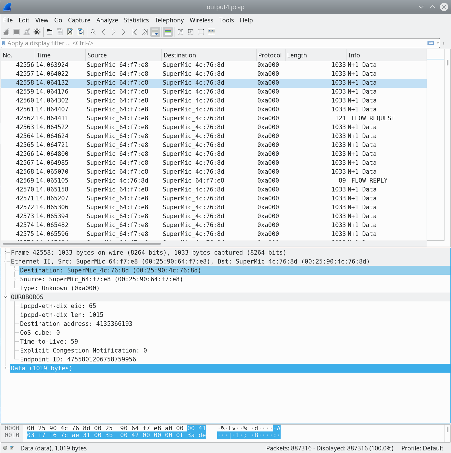
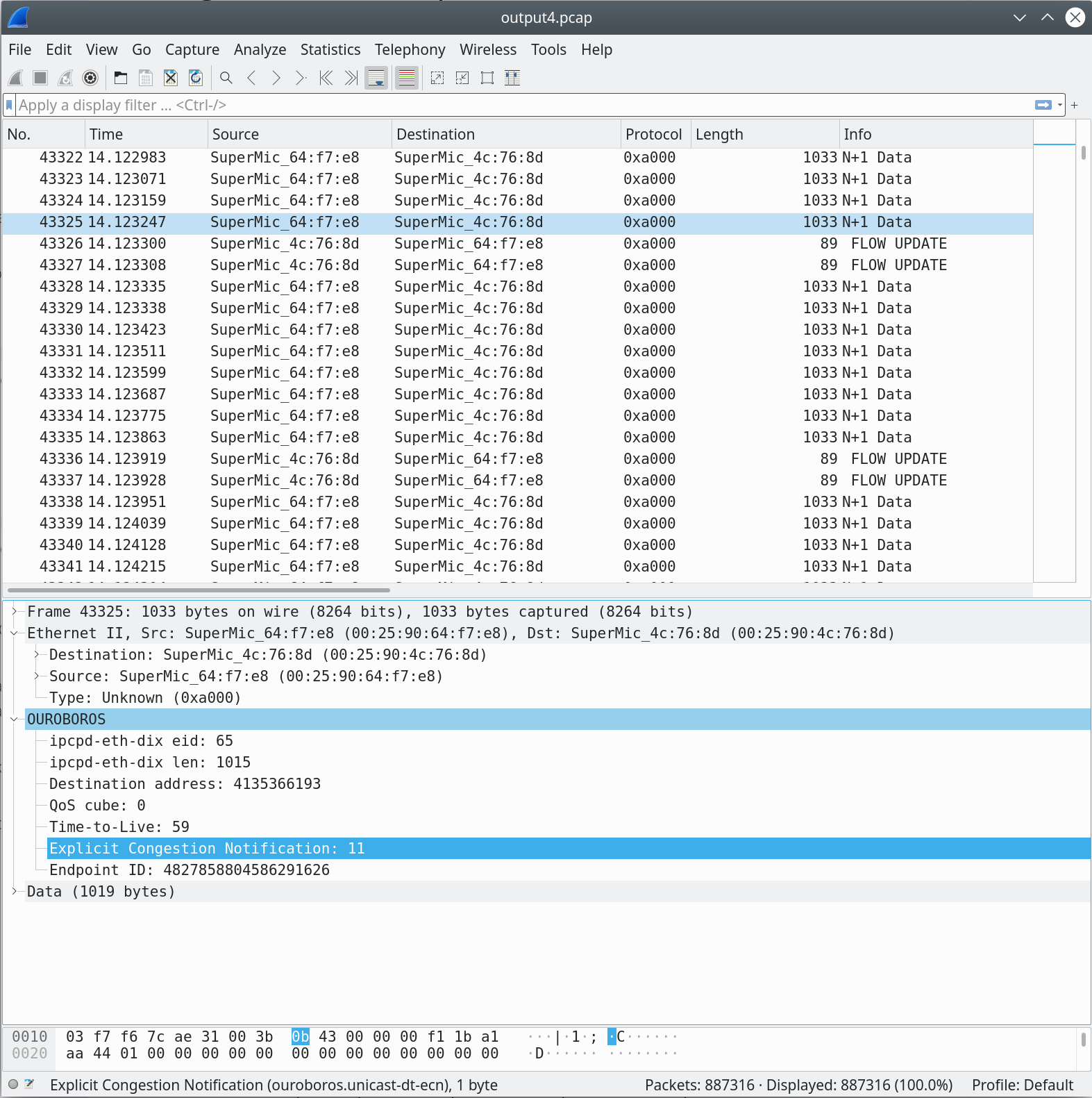
We will first have a look at packets captured around the point in time where the second (red) flow enters the network, about 14 seconds into the capture. The “N+1 Data” packets in the image above all belong to the green flow. The ocbr tool that we use sends 1000-byte data units that are zeroed-out. The packet captured on the wire is 1033 bytes in length, so we have a protocol overhead of 33 bytes⁵. We can break this down to:

        ETHERNET II HEADER               / 14 /
   6 bytes Ethernet II dst
   6 bytes Ethernet II src
   2 bytes Ethernet II Ethertype
        OUROBOROS ETH-DIX HEADER          / 4 /
   2 bytes eid
   2 byte  len
        OUROBOROS UNICAST NETWORK HEADER / 15 /
   4 bytes DST
   1 byte  QOS
   1 byte  TTL
   1 byte  ECN
   8 bytes EID
 ---    TOTAL                            / 33 /
  33 bytes

The Data (1019 bytes) reported by wireshark is what Ethernet II sees as data, and thus includes the 19 bytes for the two Ouroboros headers. Note that DST length is configurable, currently up to 64 bits.

Now, let’s have a brief look at the values for these fields. The eid is 65, this means that the data-transfer flow established between the unicast IPCPs on the router and the server (uni-r and uni-s in our experiment figure) is identified by endpoint id 65 in the eth-dix IPCP on the Server machine. The len is 1015. Again, no surprises, this is the length of the Ouroboros unicast network header (15 bytes) + the 1000 bytes payload.

DST, the destination address is 4135366193, a 32-bit address that was randomly assigned to the uni-s IPCP. The QoS cube is 0, which is the default best-effort QoS class. TTL is 59. The starting TTL is configurable for a layer, the default is 60, and it was decremented by 1 in the uni-r process on the router node. The packet experienced no congestion (ECN is 0), and the endpoint ID is a 64-bit random number, 475…56. This endpoint ID identifies the flow endpoint for the ocbr server.

The flow request

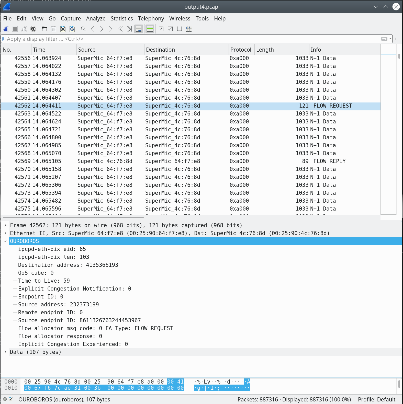
The first “red” packet that was captured is the one for the flow allocation request, FLOW REQUEST⁶. As mentioned before, the endpoint ID for the flow allocator is 0.

A rather important remark is in place here: Ouroboros does not allow a UDP-like datagram service from a layer. With which I mean: fabricate a packet with the correct destination address and some known EID and dump it in the network. All traffic that is offered to an Ouroboros layer requires a flow to be allocated. This keeps the network layer in control its resources; the protocol details inside a layer are a secret to that layer.

Now, what about that well-known EID=0 for the flow allocator (FA)? And the directory (Distributed Hash Table, DHT) for that matter, which is currently on EID=1? Doesn’t that contradict the “no datagram service” statement above? Well, no. These components are part of the layer and are thus inside the layer. The DHT and FA are internal components. They are direct clients of the Data Transfer component. The globally known EID for these components is an absolute necessity since they need to be able to reach endpoints more than a hop (i.e. a flow in a lower layer) away.

Let’s now look inside that FLOW REQUEST message. We know it is a request from the msg code field⁷.

This is the only packet that contains the source (and destination) address for this flow. There is a small twist, this value is decoded with different endianness than the address in the DT protocol output (probably a bug in my dissector). The source address 232373199 in the FA message corresponds to the address 3485194509 in the DT protocol (and in the experiment image at the top): the source of our red flow is the “Client 2” node. Since this is a FLOW REQUEST, the remote endpoint id is not yet known, and set to 0[^8. The source endpoint ID – a 64-bit randomly generated value unique to the source IPC process⁸ – is sent to the remote. The other fields are not relevant for this message.

The flow reply

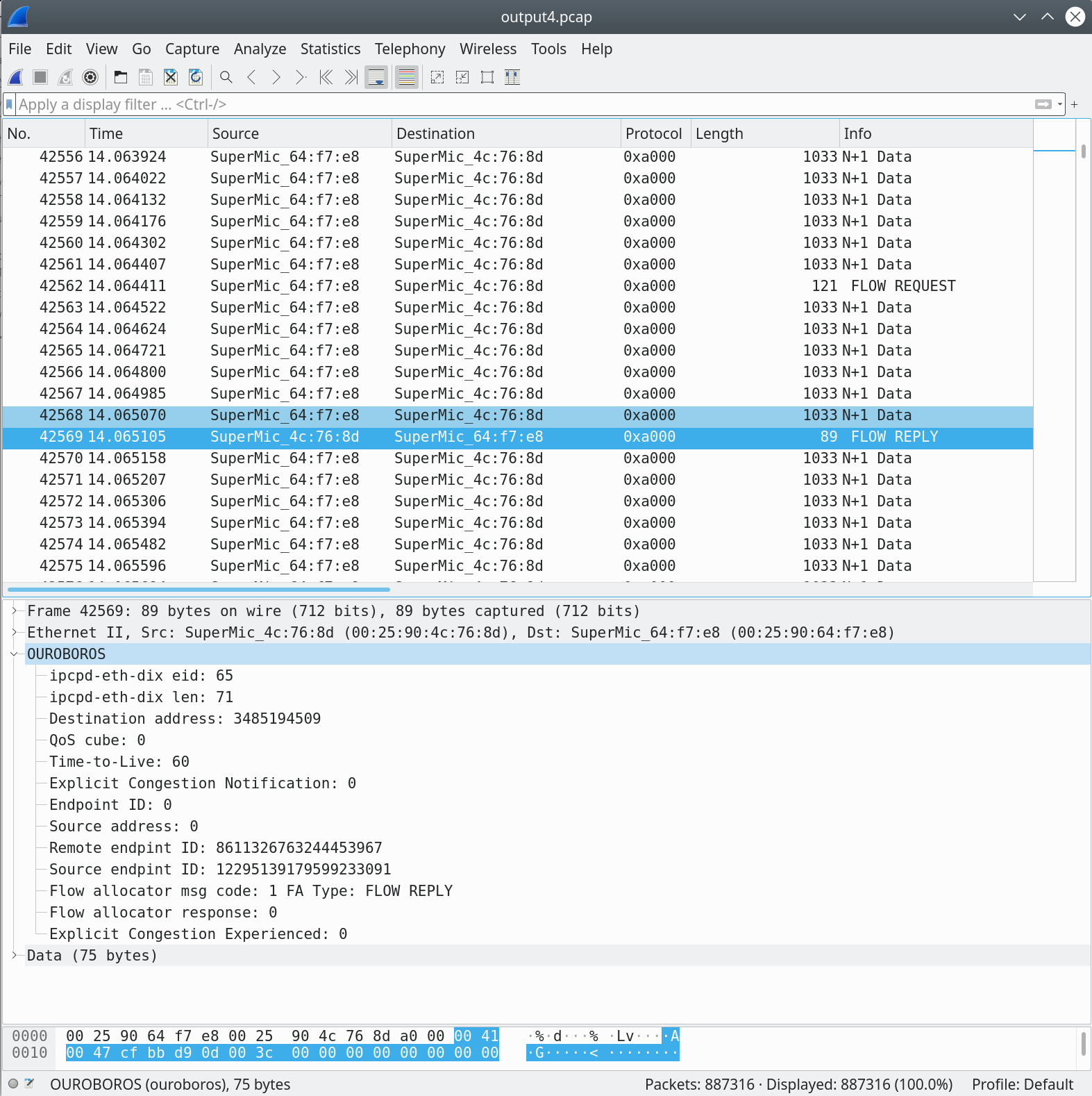
Now, the FLOW REPLY message for our request. It originates our machine, so you will notice that the TTL is the starting value of 60. The destination address is what we sent in our original FLOW REQUEST – add some endianness shenanigans. The FLOW REPLY mesage response sends the newly generated source endpoint⁹ ID, and this packet is the only packet that contains both endpoint IDs for this flow.

Congestion / flow update

Now a quick look at the congestion avoidance mechanisms. The information for the Additive Increase / Multiple Decrease algorithm is gathered from the ECN field in the packets. When both flows are active, they experience congestion since the requested bandwidth from the two ocbr clients (180Mbit) exceeds the 100Mbit link, and the figure above shows a packet marked with an ECN value of 11.

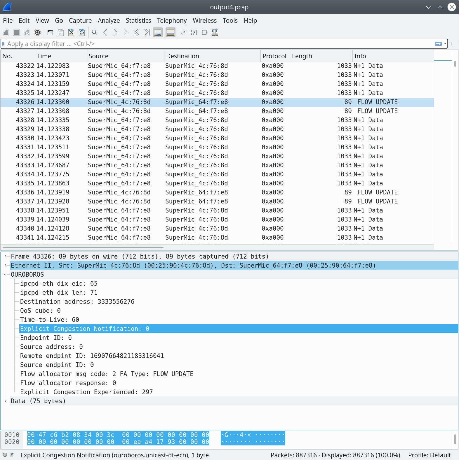
When the packets on a flow experience congestion, the flow allocator at the endpoint (the one our uni-s IPCP) will update the sender with an ECE Explicit Congestion Experienced value; in this case, 297. The higher this value, the quicker the sender will decrease its sending rate. The algorithm is explained a bit in my previous post.

That’s it for today’s post, I hope it provides some new insights how Ouroboros works. As always, stay curious.

Dimitri

• ← Previous
Next →