Congestion avoidance in Ouroboros
The upcoming 0.18 version of the prototype has a bunch of big additions coming in, but the one that I’m most excited about is the addition of congestion avoidance. Now that the implementation is reaching its final shape, I just couldn’t wait to share with the world what it looks like, so here I’ll talk a bit about how it works.
Congestion avoidance
Congestion avoidance is a mechanism for a network to avoid situations where the where the total traffic offered on a network element (link or node) systemically exceeds its capacity to handle this traffic (temporary overload due to traffic burstiness is not congestion). While bursts can be handled with adding buffers to network elements, the solution to congestion is to reduce the ingest of traffic at the network endpoints that are sources for the traffic over the congested element(s).
I won’t be going into too many details here, but there are two classes of mechanisms to inform traffic sources of congestion. One is Explicit Congestion Notification (ECN), where information is sent to the sender that its traffic is traversing a congested element. This is a solution that is, for instance, used by DataCenter TCP (DCTCP), and is also supported by QUIC. The other mechanism is implicit congestion detection, for instance by inferring congestion from packet loss (most TCP flavors) or increases in round-trip-time (TCP vegas).
Once the sender is aware that its traffic is experiencing congestion, it has to take action. A simple (proven) way is the AIMD algorithm (Additive Increase, Multiplicative Decrease). When there is no sign of congestion, senders will steadily increase the amount of traffic they are sending (Additive Increase). When congestion is detected, they will quickly back off (Multiplicative Decrease). Usually this is augmented with a Slow Start (Multiplicative Increase) phase when the senders begins to send, to reach the maximum bandwidth more quickly. AIMD is used by TCP and QUIC (among others), and Ouroboros is no different. It’s been proven to work mathematically.
Now that the main ingredients are known, we can get to the preparation of the course.
Ouroboros congestion avoidance
Congestion avoidance is in a very specific location in the Ouroboros architecture: at the ingest point of the network; it is the responsibility of the network, not the client application. In OSI-layer terminology, we could say that in Ouroboros, it’s in “Layer 3”, not in “Layer 4”.
Congestion has to be dealt with for each individual traffic source/destination pair. In TCP this is called a connection, in Ouroboros we call it a flow.
Ouroboros flows are abstractions for the most basic of packet flows. A flow is defined by two endpoints and all that a flow guarantees is that there exist strings of bytes (packets) that, when offered at the ingress endpoint, have a non-zero chance of emerging at the egress endpoint. I say ‘there exist’ to allow, for instance, for maximum packet lengths. If it helps, think of flow endpoints as an IP:UDP address:port pair (but emphatically NOT an IP:TCP address:port pair). There is no protocol assumed for the packets that traverse the flow. To the ingress and egress point, they are just a bunch of bytes.
Now this has one major implication: We will need to add some information to these packets to infer congestion indirectly or explicitly. It should be obvious that explicit congestion notification is the simplest solution here. The Ouroboros prototype (currently) allows an octet for ECN.
Functional elements of the congestion API
This section glances over the API in an informal way. A reference manual for the actual C API will be added after 0.18 is in the master branch of the prototype. The most important thing to keep in mind is that the architecture dictates this API, not any particular algorithm for congestion that we had in mind. In fact, to be perfectly honest, up front I wasn’t 100% sure that congestion avoidance was feasible without adding additional fields fields to the DT protocol, such as a packet counter, or sending some feedback for measuring the Round-Trip Time (RTT). But as the algorithm below will show, it can be done.
When flows are created, some state can be stored, which we call the congestion context. For now it’s not important to know what state is stored in that context. If you’re familiar with the inner workings of TCP, think of it as a black-box generalization of the tranmission control block. Both endpoints of a flow have such a congestion context.
At the sender side, the congestion context is updated for each packet that is sent on the flow. Now, the only information that is known at the ingress is 1) that there is a packet to be sent, and 2) the length of this packet. The call at the ingress is thus:
update_context_at_sender <packet_length>
This function has to inform when it is allowed to actually send the packet, for instance by blocking for a certain period.
At the receiver flow endpoint, we have a bit more information, 1) that a packet arrived, 2) the length of this packet, and 3) the value of the ECN octet associated with this packet. The call at the egress is thus:
update_context_at_receiver <packet_length, ecn>
Based on this information, receiver can decide if and when to update the sender. We are a bit more flexible in what can be sent, at this point, the prototype allows sending a packet (which we call FLOW_UPDATE) with a 16-bit Explicit Congestion Experienced (ECE) field.
This implies that the sender can get this information from the receiver, so it knows 1) that such a packet arrived, and 2) the value of the ECE field.
update_context_at_sender_ece <ece>
That is the API for the endpoints. In each Ouroboros IPCP (think ‘router’), the value of the ECN field is updated.
update_ecn_in_router <ecn>
That’s about as lean as as it gets. Now let’s have a look at the algorithm that I designed and implemented as part of the prototype.
The Ouroboros multi-bit Forward ECN (MB-ECN) algorithm
The algorithm is based on the workings of DataCenter TCP (DCTCP). Before I dig into the details, I will list the main differences, without any judgement.
The rate for additive increase is the same constant for all flows (but could be made configurable for each network layer if needed). This is achieved by having a window that is independent of the Round-Trip Time (RTT). This may make it more fair, as congestion avoidance in DCTCP (and in most – if not all – TCP variants), is biased in favor of flows with smaller RTT1.
Because it is operating at the flow level, it estimates the actual bandwidth sent, including retransmissions, ACKs and what not from protocols operating on the flow. DCTCP estimates bandwidth based on which data offsets are acknowledged.
The algorithm uses 8 bits to indicate the queue depth in each router, instead of a single bit (due to IP header restrictions) for DCTCP.
MB-ECN sends a (small) out-of-band FLOW_UPDATE packet, DCTCP updates in-band TCP ECN/ECE bits in acknowledgment (ACK) packets. Note that DCTCP sends an immediate ACK with ECE set at the start of congestion, and sends an immediate ACK with ECE not set at the end of congestion. Otherwise, the ECE is set accordingly for any “regular” ACKs.
The MB-ECN algorithm can be implemented without the need for dividing numbers (apart from bit shifts). At least in the linux kernel implementation, DCTCP has a division for estimating the number of bytes that experienced congestion from the received acks with ECE bits set. I’m not sure this can be avoided2.
Now, on to the MB-ECN algorithm. The values for some constants presented here have only been quickly tested; a lot more scientific scrutiny is definitely needed here to make any statements about the performance of this algorithm. I will just explain the operation, and provide some very preliminary measurement results.
First, like DCTCP, the routers mark the ECN field based on the outgoing queue depth. The current minimum queue depth to trigger and ECN is 16 packets (implemented as a bit shift of the queue size when writing a packet). We perform a logical OR with the previous value of the packet. If the width of the ECN field would be a single bit, this operation would be identical to DCTCP.
At the receiver side, the context maintains two state variables.
The floating sum (ECE) of the value of the (8-bit) ECN field over the last 2N packets is maintained (currently N=5, so 32 packets). This is a value between 0 and 28 + 5 - 1.
The number of packets received during a period of congestion. This is just for internal use.
If th ECE value is 0, no actions are performed at the receiver.
If this ECE value becomes higher than 0 (there is some indication of start of congestion), an immediate FLOW_UPDATE is sent with this value. If a packet arrives with ECN = 0, the ECE value is halved.
For every increase in the ECE value, an immediate update is sent.
If the ECE value remains stable or decreases, an update is sent only every M packets (currently, M = 8). This is what the counter is for.
If the ECE value returns to 0 after a period of congestion, an immediate FLOW_UPDATE with the value 0 is sent.
At the sender side, the context keeps track of the actual congestion window. The sender keeps track of:
The current sender ECE value, which is updated when receiving a FLOW_UPDATE.
A bool indicating Slow Start, which is set to false when a FLOW_UPDATE arrives.
A sender_side packet counter. If this exceeds the value of N, the ECE is reset to 0. This protects the sender from lost FLOW_UPDATES that signal the end of congestion.
The window size multiplier W. For all flows, the window starts at a predetermined size, 2W ns. Currently W = 24, starting at about 16.8ms. The power of 2 allows us to perform operations on the window boundaries using bit shift arithmetic.
The current window start time (a single integer), based on the multiplier.
The number of packets sent in the current window. If this is below a PKT_MIN threshold before the start of a window period, the new window size is doubled. If this is above a PKT_MAX threshold before the start of a new window period, the new window size is halved. The thresholds are currently set to 8 and 64, scaling the window width to average sending ~36 packets in a window. When the window scales, the value for the allowed bytes to send in this window (see below) scales accordingly to keep the sender bandwidth at the same level. These values should be set with the value of N at the receiver side in mind.
The number bytes sent in this window. This is updated when sending each packet.
The number of allowed bytes in this window. This is calculated at the start of a new window: doubled at Slow Start, multiplied by a factor based on sender ECE when there is congestion, and increased by a fixed (scaled) value when there is no congestion outside of Slow Start. Currently, the scaled value is 64KiB per 16.8ms.
There is one caveat: what if no FLOW_UPDATE packets arrive at all? DCTCP (being TCP) will timeout at the Retransmission TimeOut (RTO) value (since its ECE information comes from ACK packets), but this algorithm has no such mechanism at this point. The answer is that we currently do not monitor flow liveness from the flow allocator, but a Keepalive or Bidirectional Forwarding Detection (BFD)-like mechanism for flows should be added for QoS maintenance, and can serve to timeout the flow and reset it (meaning a full reset of the context).
MB-ECN in action
From version 0.18 onwards3, the state of the flow – including its congestion context – can be monitored from the flow allocator statics:
$ cat /tmp/ouroboros/unicast.1/flow-allocator/66
Flow established at:              2020-12-12 09:54:27
Remote address:                                 99388
Local endpoint ID:                2111124142794211394
Remote endpoint ID:               4329936627666255938
Sent (packets):                               1605719
Sent (bytes):                              1605719000
Send failed (packets):                              0
Send failed (bytes):                                0
Received (packets):                                 0
Received (bytes):                                   0
Receive failed (packets):                           0
Receive failed (bytes):                             0
Congestion avoidance algorithm:         Multi-bit ECN
Upstream congestion level:                          0
Upstream packet counter:                            0
Downstream congestion level:                       48
Downstream packet counter:                          0
Congestion window size (ns):                    65536
Packets in this window:                             7
Bytes in this window:                            7000
Max bytes in this window:                       51349
Current congestion regime:         Multiplicative dec
I ran a quick test using the ocbr tool (modified to show stats every 100ms) on a jFed testbed using 3 Linux servers (2 clients and a server) in star configuration with a ‘router’ (a 4th Linux server) in the center. The clients are connected to the ‘router’ over Gigabit Ethernet, the link between the ‘router’ and server is capped to 100Mb using ethtool4.
Output from the ocbr tool:
Flow   64:       998 packets (      998000 bytes)in       101 ms  => 9880.8946 pps,   79.0472 Mbps
Flow   64:      1001 packets (     1001000 bytes)in       101 ms  => 9904.6149 pps,   79.2369 Mbps
Flow   64:       999 packets (      999000 bytes)in       101 ms  => 9882.8697 pps,   79.0630 Mbps
Flow   64:       998 packets (      998000 bytes)in       101 ms  => 9880.0143 pps,   79.0401 Mbps
Flow   64:       999 packets (      999000 bytes)in       101 ms  => 9887.6627 pps,   79.1013 Mbps
Flow   64:       999 packets (      999000 bytes)in       101 ms  => 9891.0891 pps,   79.1287 Mbps
New flow.
Flow   64:       868 packets (      868000 bytes)in       102 ms  => 8490.6583 pps,   67.9253 Mbps
Flow   65:       542 packets (      542000 bytes)in       101 ms  => 5356.5781 pps,   42.8526 Mbps
Flow   64:       540 packets (      540000 bytes)in       101 ms  => 5341.5105 pps,   42.7321 Mbps
Flow   65:       534 packets (      534000 bytes)in       101 ms  => 5285.6111 pps,   42.2849 Mbps
Flow   64:       575 packets (      575000 bytes)in       101 ms  => 5691.4915 pps,   45.5319 Mbps
Flow   65:       535 packets (      535000 bytes)in       101 ms  => 5291.0053 pps,   42.3280 Mbps
Flow   64:       561 packets (      561000 bytes)in       101 ms  => 5554.3455 pps,   44.4348 Mbps
Flow   65:       533 packets (      533000 bytes)in       101 ms  => 5272.0079 pps,   42.1761 Mbps
Flow   64:       569 packets (      569000 bytes)in       101 ms  => 5631.3216 pps,   45.0506 Mbps
With only one client running, the flow is congestion controlled to about ~80Mb/s (indicating the queue limit at 16 packets may be a bit too low a bar). When the second client starts sending, both flows go quite quickly (at most 100ms) to a fair state of about 42 Mb/s.
The IO graph from wireshark shows a reasonably stable profile (i.e. no big oscillations because of AIMD), when switching the flows on the clients on and off which is on par with DCTCP and not unexpected keeping in mind the similarities between the algorithms:
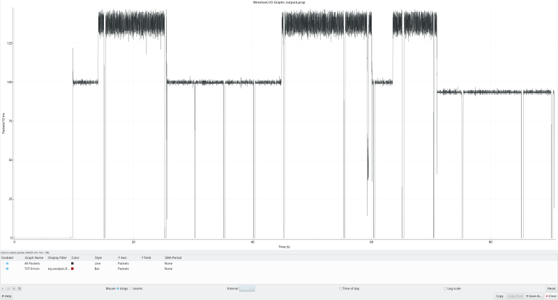
The periodic “gaps” were not seen at the ocbr endpoint applicationand may have been due to tcpdump not capturing everything that those points, or possibly a bug somewhere.
As said, a lot more work is needed analyzing this algorithm in terms of performance and stability5. But I am feeling some excitement about its simplicity and – dare I say it? – elegance.
Stay curious!
Dimitri
Additive Increase increases the window size with 1 MSS each RTT. Slow Start doubles the window size each RTT.
[return]- I’m pretty sure the kernel developers would if they could. [return]
- Or the current “be” branch for the less patient. [return]
Using Linux traffic control (
[return]tc) to limit traffic adds kernel queues and may interfere with MB-ECN.- And the prototype implementation as a whole! [return]