Metrics Exporters
Ouroboros metrics
A collection of observability tools for exporting and visualising metrics collected from Ouroboros.
Currently has one very simple exporter for InfluxDB, and provides additional visualization via grafana.
More features will be added over time.
Requirements:
Ouroboros version >= 0.18.3
InfluxDB OSS 2.0, https://docs.influxdata.com/influxdb/v2.0/
python influxdb-client, install via
pip install 'influxdb-client[ciso]'
Optional requirements:
Grafana, https://grafana.com/
Setup
Install and run InfluxDB and create a bucket in influxDB for exporting Ouroboros metrics, and a token for writing to that bucket. Consult the InfluxDB documentation on how to do this, https://docs.influxdata.com/influxdb/v2.0/get-started/#set-up-influxdb.
To use grafana, install and run grafana open source, https://grafana.com/grafana/download https://grafana.com/docs/grafana/latest/?pg=graf-resources&plcmt=get-started
Go to the grafana UI (usually http://localhost:3000) and set up InfluxDB as your datasource: Go to Configuration -> Datasources -> Add datasource and select InfluxDB Set “flux” as the Query Language, and under “InfluxDB Details” set your Organization as in InfluxDB and set the copy/paste the token for the bucket to the Token field.
To add the Ouroboros dashboard, select Dashboards -> Manage -> Import
and then either upload the json file from this repository in
dashboards-grafana/general.json
or copy the contents of that file to the “Import via panel json” textbox and click “Load”.
Run the exporter:
Clone the repository:
git clone https://ouroboros.rocks/git/ouroboros-metrics
cd ouroboros-metrics
cd exporters-influxdb/pyExporter/
Edit the config.ini.example file and fill out the InfluxDB information (token, org). Save it as config.ini.
then run oexport.py
python oexport.py
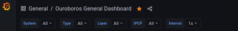
Overview of Grafana general dashboard for Ouroboros
The grafana dashboard allows you to explore various aspects of Ouroboros running on your local or remote systems. As the prototype matures, more and more metrics will become available.
Variables
At the top, you can set a number of variables to restrict what is seen on the dashboard:
- System allows you to specify a set of host/node/devices in the network:
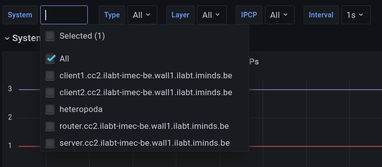
The list will contain all hosts that put metrics in the InfluxDB database in the last 5 days (Unfortunaly there seems to be no current option to restrict this to the current selected time range).
- Type allows you to select metrics for a certain IPCP type
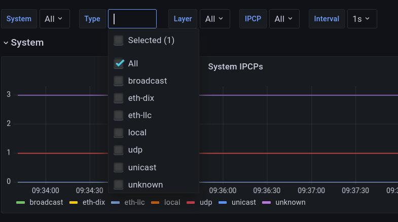
As you can see, all Ouroboros IPCP types are there, with unclusion of an UNKNOWN type. This may briefly pop up when the metric is misread by the exporter.
Layer allows you to restrict the metrics to a certain layer
IPCP allows to restrict metrics to a certain IPCP
Interval allows to select a window in which metrics are aggregated.
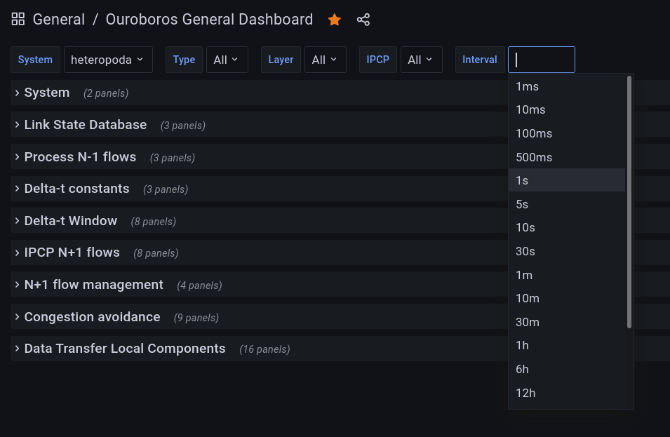
Metrics will be aggregated from the actual exporter values (e.g. mean or last value) that fall in this interval. This interval should thus be larger than the exporter interval to ensure that each window has enough raw data.
Panels
As you can see in the image above, the dashboard is subdivided in a bunch of panels, each of which focuses on some aspect of the prototype.
System
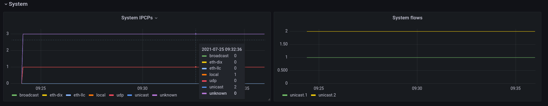
The system panel shows the number of IPCPs and known IPCP flows in all monitored systems as a stacked series. This system is running a small test with 3 IPCPs (2 unicast IPCPs and a local IPCP) with a single flow between oping server/client(which has one endpoint in each IPCP, so it shows 2 because this small test runs on a single host). The colors on the graphs are sometimes not matching the labels, which is a grafana issue that I hope will get fixed soon.
Link State Database
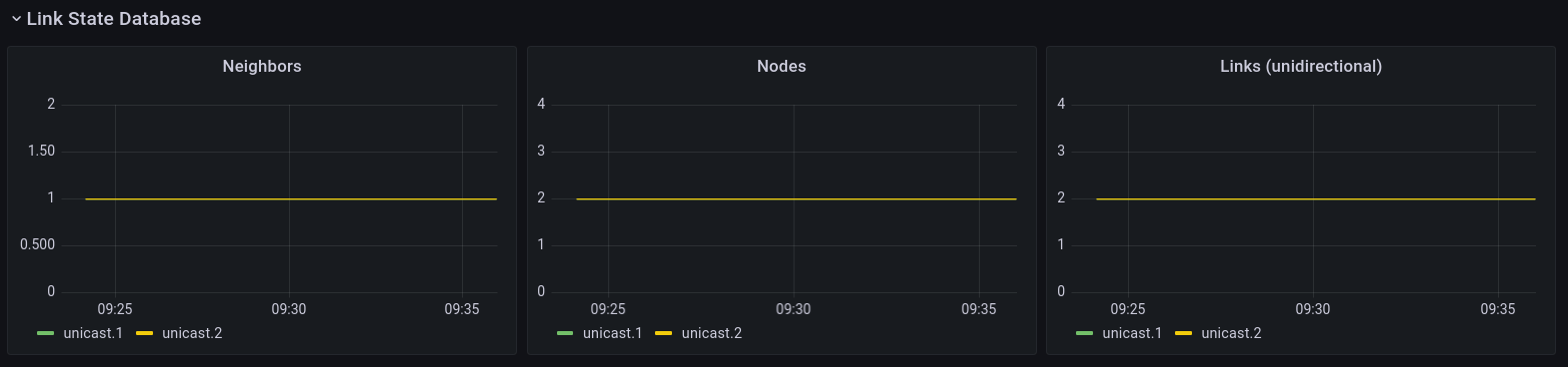
The Link State Database panel shows the knowledge each IPCP has about the network routing area(s) it is in. The example has 2 IPCPs that are directly connected, so each knows 1 neighbor (the other IPCP), 2 nodes, and two links (each unidirectional arc in the topology graph is counted).
Process N-1 flows
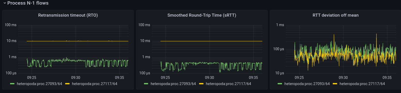
This is the first panel that deals with the Flow-and-Retransmission Control Protocol (FRCP). It shows metrics for the flows between the applications (this is not the same flow as the data transfer flow above, which is between the IPCPs). This panel shows metrics relating to retransmission. The first is the current retransmission timeout, i.e. the time after which a packet will be retranmitted. This is calculated from the smoothed round-trip time and its estimated deviation (well below 1ms), as estimated by FRCP.
The flow is created by the oping application that is pinging at a 10ms interval with packet retransmission enabled (so basically a service equivalent as running ping over TCP). The main difference with TCP is that Ouroboros flows are between the applications themselves. The oping server immediately responds to the client, so the client sees a response time well below 1 ms1. The server, however, sees the client sending a packet only every 10ms and its RTO is a bit over 10ms. The ACKs from the perspective of the server are piggybacked on the client’s next ping. (This is similar to TCP “delayed ACK”, the timer in Ouroboros is set to 10ms, so if I would ping at 1 second intervals over a flow with FRCP enabled, the server would also see a 10ms Round-trip time).
Delta-t constants
The second panel to do with FRCP are the Delta-t constants. Delta-t is the protocol on which FRCP is based. Right now, they are only configurable at compile time, but in the future they will probably be configurable using fccntl().
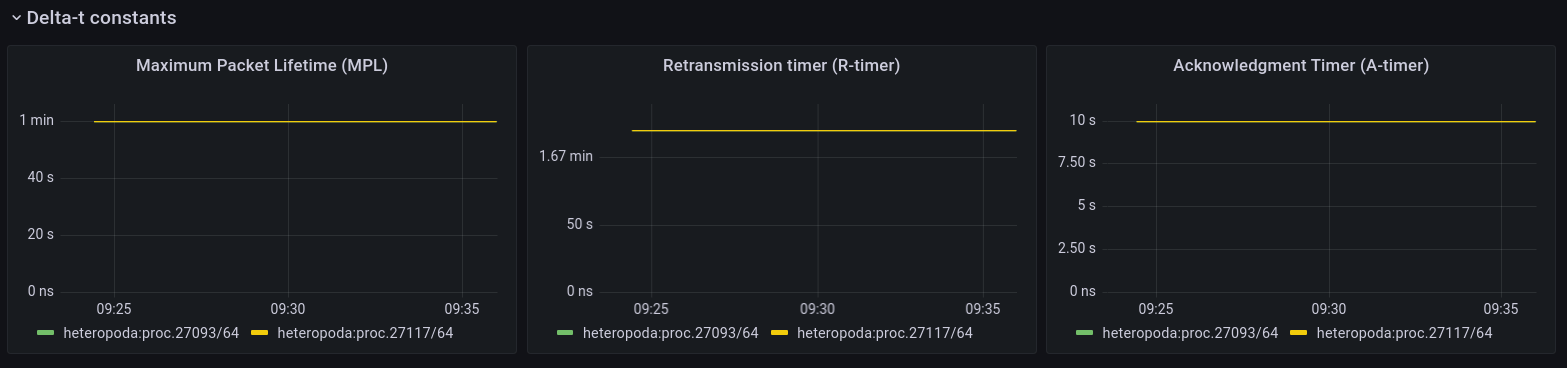
A quick refresher on these Delta-t timers:
Maximum Packet Lifetime (MPL) is the maximum time a packet can live in the network, default is 1 minute.
Retransmission timer ® is the maximum time which a retransmission for a packet may be sent by the sender. The default is 2 minutes. The first retransmission will happen after RTO, then 2 * RTO, 4* RTO and so on with an exponential back-off, but no packets will be sent after R has expired. If this happens, the flow is considered failed / down.
Acknowledgment timer (A) is the maximum time which an packet may be acknowledged by the receiver. Default is 10 seconds. So a packet may be acknowledged immediately, or after 10 milliseconds, or after 4 seconds, but not any more after 10 seconds.
Delta-t window
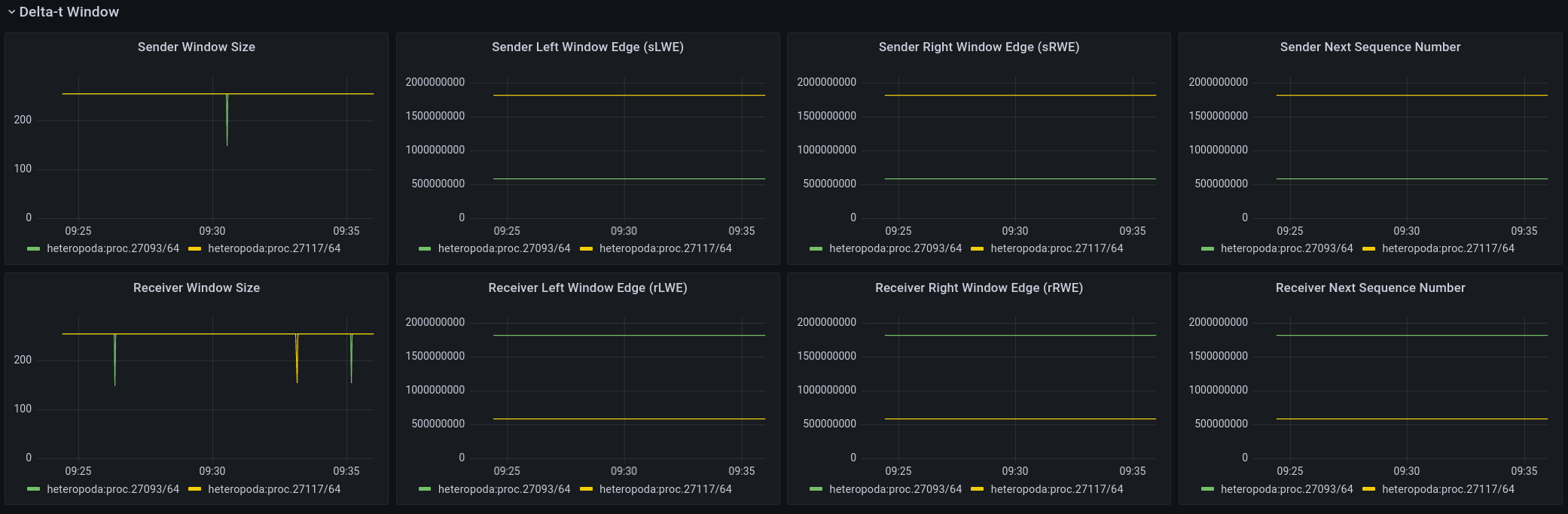
The third and (at least at this point) last panel related to FRCP is the window panel that shows information regarding Flow Control. FRCP flow control tracks the number of packets in flight. These are the packets that were sent by the sender, but have not been read/acknowledged yet by the receiver. Each packet is numbered sequentially starting from a random value. The default maximum window size is currently 256 packets.
IPCP N+1 flows
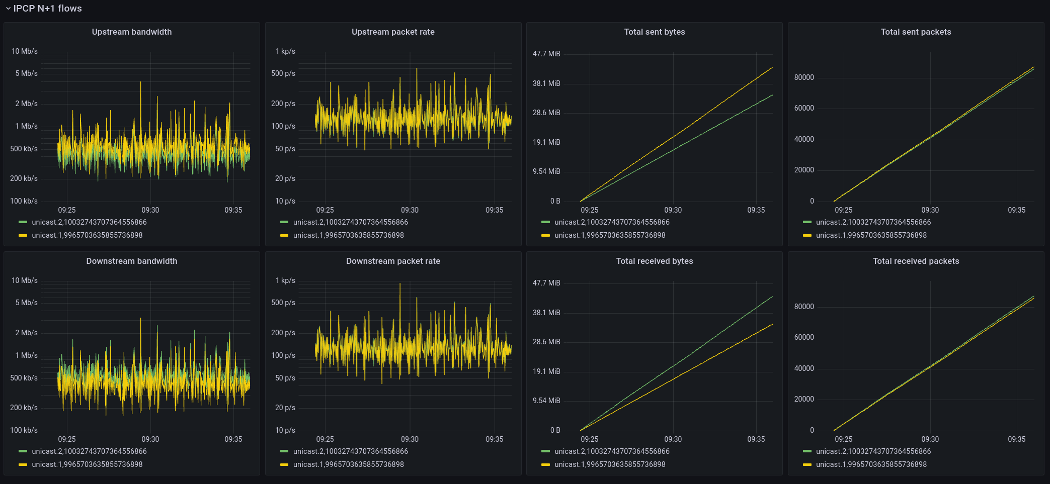
These graphs show basic statistics from the point of view of the IPCP that is serving the application flow. It shows upstream and downstream bandwidth and packet rates, and total sent and received packets/bytes.
N+1 Flow Management
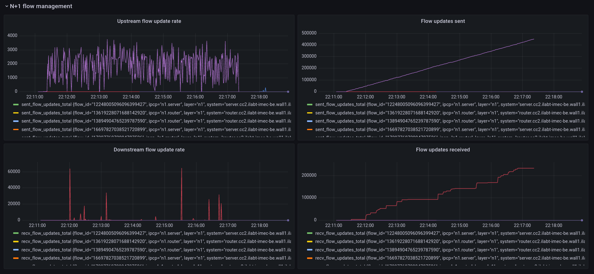
These 4 panels show the management traffic sent by the flow allocators. Currently this traffic is only related to congestion avoidance. The example here is taken from a jFed experiment during a period of congestion. The receiver IPCP monitors packets for congestion markers and it will send an update to the source IPCP to inform it to slow down. It shows the rate of flow updates for multi-bit Explicit Congestion Notification. As you can see, there is still an issue where the receiver is not receiving all the flow updates and there is a lot of jitter and burstiness at the receiver side for these (small) packets. I’m working on fixing this.
Congestion Avoidance
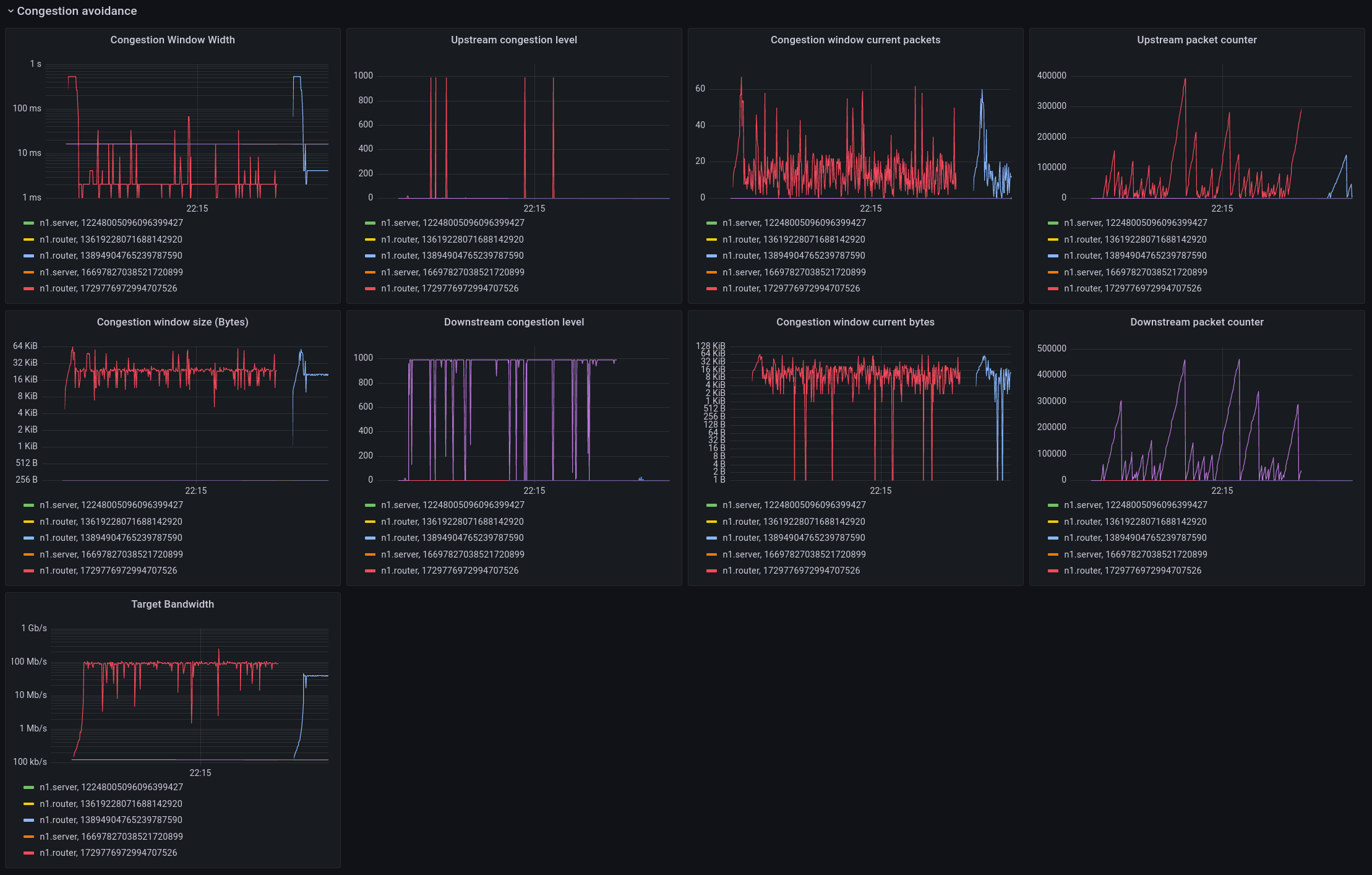
This is a more detailed panel that shows the internals of the MB-ECN congestion avoidance algorithm.
The left side shows the congestion window width, which is the timeframe over which the algorithm is averaging bandwidth. This scales with the packet rate, as there have to be enough packets in the window to make a reasonable measurement. Biggest change compared to TCP is that this window width is independent of RTT. The congestion algorithm then sets a target for the maximum number of bytes to send within this window (congestion window size). The division of the number of bytes that can be sent and the size of the windows yields the target bandwidth. The congestion was caused by a 100Mbit link, and the target set by the algorithm is quite near this value. The congestion level is a quantity that controls the rate at which the window scales down when there is congestion. This upstream/downstream view should be as close as possible to identical, the reason they are not is because of the jitter and loss in the flow updates as observed above. Work in progress.
The graphs also show the number of packets and bytes in the current congestion window. The default target is set to min 8 and max 64 packets within the congestion window before it scales up/down.
And finally, the upstream packet counters shows the number of packets sent without receiving a congestion update from the receiver, and the downstream packet counter shows the number of packets received since the last time there was no congestion.
Data transfer local components
The last panel shows the (management) traffic sent and received by the IPCP internal as measured by the forwarding engine (Data transfer).
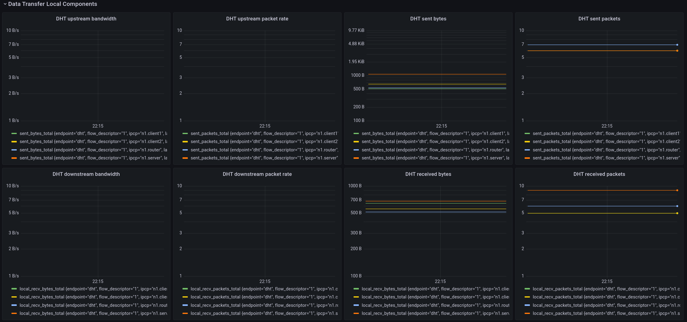
The components that are current shown on this panel are the DHT and the Flow Allocator. As you can see, the DHT didn’t do much during this interval. That’s because it is only needed for name-to-address resolution and it will only send/receive packets when an address is resolved or when it needs to refresh its state, which happens only once every 15 minutes or so.
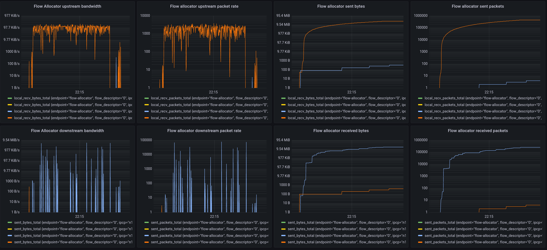
The bottom part of the local components is dedicated to the flow allocator. During the monitoring period, only flow updates were sent, so this is the same data as shown in the flow management traffic, but from the viewpoint of the forwarding element in the IPCP, so it shows actual bandwidth in addition to the packet rates.
If this still seems high, disabling CPU “C-states” and tuning the kernel for low latency can reduce this to a few microseconds.
[return]